When there are linear constraints, interval arithmetic (like the one used in FBBT) can be taken one step further.
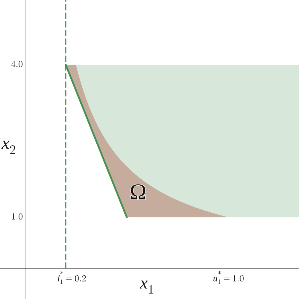
Take the linear constraint \(-10x_1-x_2 \leq -6\) for \(x_2 \in [1,4]\) of problem \(P\) corresponding to the green area in Figure 4.
We can rewrite this inequality as \(x_1 \geq \frac{6-x_2}{10}\), and apply interval arithmetic to bound the function
\(\frac{6-x_2}{10}\), between 0.2 and 0.5 (see example in FBBT section), to obtain the inequality \(x_1 \geq \frac{6-x_2}{10} \geq 0.2\).
Therefore, we can change the bounds of \(x_1\) in \(P\) from \([0,4]\) to \([0.2,4]\). In this case, the lower bound found using constraint propagation corresponds to the tightest bound possible for \(x_1\) (\(l^*_1\) in Figure 4). Note that if the original upper bound of \(x_1\) was \(0.1\) instead of \(4\) we could have concluded that the problem was infeasible.
Putting this into Practice
The idea is to apply constraint propagation to all the linear constraints in the problem. In general, using a linear equality constraint
\(\sum_{i=1}^{n}a_{i}x_{i}=b\)
we can bound all variables \(x_{i}) ((i =1, \dots,n)\) from below and above (depending on the sign of the coefficient \(a_i\)) by the values
\[\frac{1}{a_{i}}(b-\sum_{j=1\\ j\neq i}^{n}\min(a_j l_j,a_j u_j)),\]
and
\[\frac{1}{a_{i}}(b-\sum_{{j=1\\j\neq i}}^{n}\max(a_{j}l_j,a_{j}u_j)),\]
where \(l_j \leq x_j \leq u_j \forall j \neq i\). These values often provide bounds for \(x_i\) which are tighter than the original lower and upper bounds \(l_i\) and \(u_i\), or can provide us with a certificate of infeasibility for the problem.
Note that for linear constraints of lesser or greater sense you can derive the corresponding one-sided bounds.
One iteration of the constraint propagator consists of applying the technique once to every linear constraint.