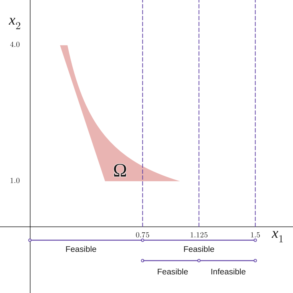
The basic idea of FBBT is to find intervals for the variables where no feasible point can be found. Consider the intervals \(I_1 = [0,0.75]\) and \(I_2 = [0.75,1.5]\) for the variable \(x_1\) for problem \(P\). We know that there are feasible points \(x_1, x_2\) for \(P\) if \(x_1 \in I_2\), and therefore we can not discard this interval.
If we repeat this procedure for \(I_2\), e.g., divide the interval \([0.75,1.5]\) into \([0.75,1.125]\) and \([1.125,1.5]\), we will see that the interval \([1.125,1.5]\) does not have any feasible points, and therefore we can discard it and update the upper bound for \(x_1\) from 1.5 to 1.125 (see Figure 3).
The question is how can we know when to discard an interval. FBBT uses interval arithmetic to answer this question.
Consider the function \(f(x_1) = 2x_1 + 3\) with \(x_1 \in [1,2]\). Given that (f) is an increasing function on this domain, we can bound it by taking the minimum and maximum of the interval \([1,2]: f(1)=5 \leq f(x_1) \leq 7= f(2)\).
Similarly, the function \(g(x_1,x_2) = x_1x_2\ \) with \(x_1 \in [1.125,1.5]\) and \(x_2 \in [1,4]\) is also increasing with respect to both variables in the domain, and therefore it can be bounded using the extremes of the intervals, i.e., \(g(1.125,1)=1.125\leq g(x_1,x_2) \leq 6 = g(1.5,4)\). Interval arithmetic can be used for other types of structures too.
Taking the constraint \(x_1x_2 \leq 1\) in problem (P) and the bounds found using interval arithmetic for the function \(g(x_1,x_2)\), we notice that \(g\) is bounded below by 1.125 if we restrict \(x_1\) to the interval \(I_2 = [1.125,1.5]\).
Therefore, the constraint is infeasible in the interval (as the upper bound of the constraint is 1), \(I_2\) can be discarded, and we can reduce the domain of \(x_1\) in \(\Omega\) from \([0,1.5]\) to \([0,1.125]\).
Putting this into Practice
Let \({x_i}\in{[l_i,u_i]}\) (\(i=1,\dots,n\)), \(f(x_1,\dots,x_n)\) and \(UB\) be the variables, the objective function and a known upper bound of a problem respectively.
Similarly, w.l.o.g. let \({c_j(x_1,\dots,x_n)}\leq{b_j}\) for \(j=1,\dots,m\) be the constraints of the problem (all the arguments that will follow can be generalised for greater than inequalities as well as equalities in the constraints). Then, if \({I}\subset{[l_i,u_i]}\), let \(g^{i,I}_L\) and \(g^{i,I}_U\) be the lower and upper bounds for any function \(g(x_1,\dots,x_n)\) calculated using interval arithmetic on \({x_i}\in{I}\).
If lower and upper bounds are calculated for every function using \({x_i}\in{I}\), then the subset \({x_i}\in{I}\) can be discarded from the feasible set if:
The lower bound of the objective function is larger than the known upper bound, i.e, \( {f^{i,I}_L}>UB \) (in this case, we know that the value of \(x_i\) in an optimal solution cannot be contained in the subset \(I\)).
The lower bound of a constraint is larger than the right hand side, i.e., \({{c_j}_{L}^{i,I}}>b_j \) (in this case, the smallest value of the constraint for \({x_i}\in{I}\) is larger than \(b_j\), which implies that the problem is infeasible for any point with \({x_i}\in{I}\)).
Octeract Engine applies the previous methodology by evaluating different subsets of the intervals for the variables and updating the lower and upper bounds of the variable. In particular, for every variable \({x_i}\in{[l_i,u_i]}\), the lower bound \(l_i\) is updated by splitting the original interval in two subintervals \(I_1=[l_i,M]\) and \(I_2=[M,u_i]\), and determining if they can be eliminated.
If both intervals can be eliminated, then the problem is infeasible. If \(I_1\) can be eliminated but not \(I_2\), then the lower bound \(l_i\) is set equal to \(M\), and the process is repeated. Similarly, if \(I_1\) cannot be eliminated the process is repeated splitting \(I_1\) in two. A similar process is also done to update the upper bound \(u_i\).